Sections:
Books:
"ODEs using Matlab", 3rd ed. by Polking and Arnold (PA).
Office hours:
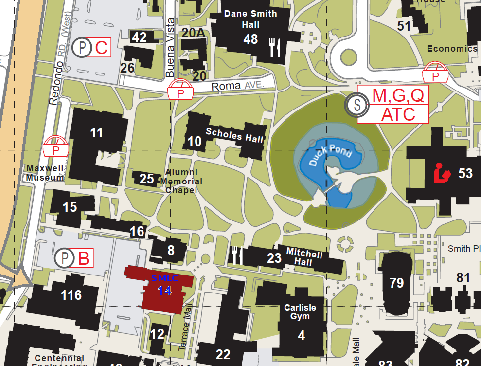
Monday, Tuesday, Wednesday 14:00-14:50. Room: SMLC 220.
How grades are assigned?
All homeworks: 100 points.Two midterm exams: 100 points each (100+100 points).
In class quizes: 50 points.
Final exam: 200 points.
Total: 550 points.
Lowest thresholds for grades (not higher than):
A = 495, B = 440, C = 380, D = 330.
All numbers without brackets correspond to BB 1st edition, in the brackets -- 2nd edition.
For example: BB 2.1(1.2): 2(3) means that if you have 1st edition you need to do BB 2.1: 2, if 2nd -- BB 1.2: 3.
| Week # | Homework problems | Due date |
|---|---|---|
| 11 |
Final Exam (Tuesday, December 11th, 7:30am) (Solution published). Quiz 09 (Tuesday, December 4th) (Solution published). Topic: method of integrating factor. Quiz 10 (Thursday, December 6th) AT THE BEGINNING OF THE CLASS (Solution published). Topic: method of undetermined coefficients. You need to be able to choose the right form for particular solution. Sample final exam problems: Sec. 2.1(1.2): 18; Sec. 2.5(2.4): 12 (find implicit analytical solution using partial fractions); Sec. 3.3(3.3): 13; Sec. 3.4(3.4): 6; Sec. 3.5(3.5): 11; Sec. 4.3(4.3): 41(reduction of order, not present in 2nd Ed., see lecture); Sec. 4.4(4.3): 39(59); Sec. 4.6(4.5): 5, 7, 28; Sec. 4.8(4.7): 17, 22; Sec. 5.6(5.6): 6; Sec. 7.2(7.2): 7. There will be 8 problems on the final exam. You can have a page (both sides) of information with you. You shall get Laplace transforms table. |
|
| 10 |
Quiz 07 (Tuesday, November 20th) (Solution published). You need to be able to determine type of a critical point of a linear system of ODEs and sketch the phase portrait. Quiz 08 (Thursday, November 29th) (Solution published). You need to be able to find critical points of NL system and analyze them. Sec.5.7(5.7): 1,2,5; Sec.7.2(7.2): 1,3,5,7,9,11. Matlab Problem: Study Example 3 on p.109ff of Polking. Redo the problem using the initial condition x_1(0)=1, x_2(0)=0. |
November 29th, 2012, class time. |
| 10 |
Second Mid-Term Exam (Tuesday, November 6th) (Solution published). You will have a table of Laplace transforms and also you can have ONE page (one side) of whatever you like. Sample problems for the exam: Sec. 4.4(4.3), p. 252(252): 35(55); Sec. 4.6(4.5), p. 271(273): 7(7); Sec. 4.8(4.7), p. 290(292): 16(16); Sec. 5.4(5.4): 8(8), 11(11); Sec. 5.6(5.6), p. 354(357): 3(3). Also the reduction of order technique is recommended for review. Quiz 06 (Thursday, November 1st) (Solution published). You need to be able to use method of variation of parameters for a second order ODE. Sec.5.2(5.2): previously you have solved problems for Section 4.6: 14,16,18 on p.270(272). For these problems (from BB 4.6) find the Laplace transform (LT) of the solution as directed on p.322(325) for problems 12-21. Then show it is the same as the LT of the solution determined on p. 270(272) (which you have got in your previous HW, returned on Thursday). BB 5.3(5.3): 6, 9-24; BB 5.4(5.4): 2,4,6,8,10; (you will need to use the techniques from BB 5.3 to find the inverse transform, as e.g. in problems 9-24 p.332(334-335)); BB 5.5(5.5): 7(7), 9(9); BB 5.6(5.6): 3(3), 7(7), 8(8). |
November 8th, 2012, class time. |
| 9 |
Quiz 05 (Thursday, October 25th) (Solution published). You need to be able to use method of undetermined coefficients. BB 4.7(4.6): 1,2,4,13,16,17,18; BB 4.8(4.7): 2, 4, 10, 12, 14. BB 5.1(5.1): 4,16,20,24; |
October 30th, 2012, class time. | 6-8 |
Quiz 04 (Thursday, October 18th) (Solution published). Topic: Homogeneous ODEs of the second order with constant coefficients. Pay attention, you have to do the problems including 4.4 (4.3) before the quiz! BB 4.1(4.1): 1-5 (give reasons); BB 4.2(4.2): 8, 10, 20, 21, 24; BB 4.3(4.3): 1, 2, 6(14), 10(4), 28(41); Supplementary material: In 2 and 6(14)b, sketch the PPP by hand. You are not asked to use PPlane. In 10b use PPlane. Required material: BB 4.4(4.3): 12(6), 14(12), 17(23), 26(42). Note that 26(42) is an extension of 14(12); Extra problem: Explain why the spirals in the context of Sec. 4.4 are always CW; BB 4.5(4.4): 1,2; BB 4.6(4.5): 2, 9, 10, 13, 14, 15, 16, 18, 27; BB 2.1(1.2): 39. |
October 23rd, 2012, class time. |
| 5 |
Quiz 03 (Tuesday, September 25th) (Solution published). Topics: Euler method, local and global errors. Exam 1 (Solution published)(Example) (Thursday, September 27th). This homework is a practice. All previous quizzes will be included as well. (1) BB 3.4(3.4): 2,7. Include a sketch of the phase plane portrait drawn by hand. (2) BB 3.4(3.4): 10. Include the general solution and a sketch of the phase plane portrait drawn by hand (3) BB 3.5(3.5): 7,8. Find the general solution and solve the IVP. No plots are required. |
September 25th, 2012, class time. |
| 3-4 |
Quiz 02 (Thursday, September 6th) (Solution published). Topics: Method of integrating factor. BB 2.8(2.7) p.113(109). Use eul.m and rk2.m from PA to check the table on 2.8.1(2.7.1). rk2.m implements the Improved Euler. I. Problem 1 p.72 Polking. You will need to download rk4 from Polking's web site. II. Follow the instructions in Problem 1b (you don't need exact solution!!!) p.72 of Polking for the IVP y'=t^2 + y^2, with y(0)=1, on [0,1]; h=.1 and .01. Can you estimate the blow up point? This problem does not have a solution in terms of elementary functions, it does have a solution in terms of Bessel functions. III. Solve the IVPs y'=y^2 and y'=1+y^2 with y(0) =1. Discuss the forward interval of existence. In this case it corresponds to where the solutions blow up. Use the direction fields to argue that the solution in II blows up in between the other two blow up points. IV. BB 3.1 (3.1): 14,16,18,22,34,38. (1) BB 3.2(3.2): 16 (22) (2) BB 3.2(3.2) and 3.3(3.3): 11 (17) p.147(150) and 9 p.162 (167) (3) BB 3.2(3.2) and 3.3(3.3): 12 (18) p.147(150) and 11 p.162 (167) and 16 p.162 (167). In 16 also find an IC such that x(t) -> 0 as t -> infinity (4) BB 3.3(3.3): 2,13,18,20; (5) BB 3.4(3.4): 3,8; In problems (2), (3), (4) and (5) use Polkings PPLANE as discussed in his Chapter 7 (PA) to draw the direction fields and phase plane portraits. |
September 18th, 2012, class time. |
| 1-2 |
Quiz 01 (Thursday, August 23rd) (Solution published). Topics: product rule, chain rule, table integrals, integration by parts. Download any version of dfield you like (dfield8 for example) and any version of pplane (pplane7 for example) from Polkings web site (see PA last page of preface and p.47) BB Sec.1.1 (1.1): 1, 3; use Matlab and dfield7 to plot dfields (see Chapter 3in PA) Solve each of the following two initial value problems and plot the solutions for several values of y_0. Then describe in a few words how the solutions resemble, and differ from, each other: 1a. y'=-y+5, y(0)=y_0; 1b. y'=-2y+5, y(0)=y_0. previous two problems do in two ways:(I)find solution and plot it using Matlab's ezplot(see p.9 in PA) (II) use Polkings dfield to obtain a plot of the dfield with several solutions BB 1.3(1.3): 1, 9, 16; use the eul.m script on page 73, do 1 step by hand to check code. BB 1.4(1.4): 8, 13, 14; BB 2.1(1.2): 13, 15, 16. For Matlab exercises show your matlab work. BE NEAT for full credit. BB 2.2(2.1): 1,9,10,12; use ezplot or fplot for graphs BB 2.5(2.4): 2,4,10,12; In problems 2 and 10 find the solution using the separable technique and partial fractions as illustrated on p.86 (82) and verify your sketch. |
September 4th, 2012, class time. |