Sections:
Books:
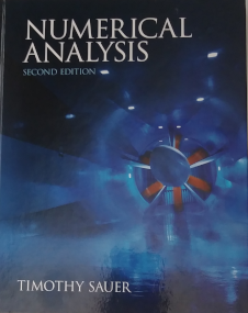
Numerical Analysis
2nd Edition, Pearson.

Additional material (by courtesy of Prof. S. Lau) can be found at the bottom of the page.
Additional Matlab tutorial by Prof. M. Nitsche.
Office hours:
TR 12:30-13:45. Room: Remote Scheduled.
How grades are assigned?
All homeworks: 250 points.Midterm exam: 125 points.
Final exam: 125 points.
Total: 500 points.
Lowest boundaries for grades (not higher than):
A = 450, B = 400, C = 350, D = 300.
Homework regulations
HW has to be typed in what ever editor you like.If you were asked to produce any output from Matlab - it has to be copied in the HW text.
If you were asked to prepare a script and use it, every Matlab script has to be printed.
If you were asked to plot something, this plot has to be printed.
Essentially, it is recommended to type all HW together with plots and cut-and-paste scripts and Matlab outputs.
| Week # | Homework problems | Due date |
|---|---|---|
| - |
Final Exam: Thursday, May 13th, 2021, 7:30-9:30am, through UNM Learn. What is covered: all topics. You need to understand and be able to use definitions and algorithms. Training set of problems: Sauer, p. 19: 0.4.1; Sauer, p. 59: 1.4.5; Sauer, p. 101: 2.4.3; Sauer, p. 198: 4.1.2, 4.1.7-9; Sauer, p. 224: 4.3.1, 4.3.2 (Using both Gramm-Schmidt process and Givens' rotations (see lectures linalg4-5)); For linear algebra in general: you need to be able to estimate number of operations necessary to complete the problem, understand sources of errors (condition number), similar to problems in Midterm; Sauer, p. 156: 3.2.1-3 (also work through problems in the Midterm); Sauer, p. 164: 3.3.1, 3.3.5, 3.3.7-8; Sauer, p. 176: 3.4.7, 3.4.12; Sauer, p. 263: 5.2.1-3 (also you shall need understanding of error dependence on a grid step); Sauer, p. 278: 5.5.1-3 (work through HW#11); Sauer, p. 252: 5.1.1, 5.1.5; Sauer, p. 321: 6.4.3 (you need to be able to use all methods we studied); In all methods which we studied you need to understand errors dependence on the parameters of methods like grid step etc. | - |
| 12 |
Homework 12 (10 Extra Credit points). Help with analytical solution. |
May 7th, 2021, |
| 11 |
Homework 11 HW11 Solution. |
April |
| 9-10 |
Homework 09-10. HW09 Solution HW10 Solution. |
April 20th, 2021, end of day. |
| - |
Midterm: March 30th, class time (Solution published). What is covered: all topics up to and including interpolation. You need to understand and be able to use definitions and algorithms. Training set of problems: HW 2: 1, 2; HW 3: 1, 4; HW 4: 1-3; HW 5: 1, 2; HW 6: 1; HW 7: 3; HW 8: 1, 4; anything else from what we studied also can be included. |
March 30th, 2021, class time. |
| 7-8 | Homework 07-8 HW07 Solution HW08 Solution. |
March 30th, 2021, end of day. |
| 5-6 | Homework 05-6 HW05 Solution HW06 Solution. |
March 4th, 2021, end of day. |
| 3-4 | Homework 03-4 HW03 Solution HW04 Solution. |
February 18th, 2021, end of day. |
| 2 | Homework 02 HW02 Solution. |
February |
| 1 | Homework 01 HW01 Solution. |
January 28th, 2021, end of day. |
Below you can find additional material.
| Week # | Lectures Notes and scripts (by courtesy of Prof. Lau) | ||
|---|---|---|---|
| YouTube playlist for lectures' recordings. | |||
| 14 | TS 6.2-6.4, Analysis of IVP solvers. Higher order ODEs, Systems of ODEs. | TS 6.4-5, Systems of ODEs, Variable time step. | |
| 14 |
Lecture 27 (quad2) Lecture 28 (quad3) TS 5.2, NewtonCotesClosedWeights.m |
Lecture 28 (quad3)
TS 5.2, 5.5. TS 6.1, Numerical Differentiation |
|
| 13 |
Lecture 25 (root4)
TS 2.7, |
Lecture 26 (quad1) , TS 5.2 | |
| 12 | TS 4.2-4.3 | Lecture 20 (linalg5) | |
| 11 |
Lecture 21 (splines1), TS 3.4 |
Lecture 22 (linalg4) , TS 4.1-4.2 | |
| 10 | Midterm |
Lecture 20 (splines1), TS 3.4 pwchermite_coeffs.m Compute coefficients defining piecewise cubic (PWC) Hermite spline. eval_pwpoly.m Evaluate piecewise defined polynomial with Horner's rule. |
|
| 9 | Lecture 14, (interp3), TS 3.2 | Lecture 15 (interp4), TS 3.3 | |
| 8 | Lecture 12 (interp1) , TS 2.5. | TS 2.5,
Lecture 13 (interp2), TS 3.2 hornernewt.m Calculation of Newton's method coefficients using Horner's rule for polynomials. |
|
| 7 |
Lecture 13 (linalg2), TS 2.3-2.4. |
Lecture 13 (linalg2) Lecture 11 (linalg3), TS 2.4. Lecture 14 (interp1) , TS 3.1 |
|
| 6 |
Lecture 11 (linalg3), TS 2.3-2.5 GE.m LU factorization without pivoting (unstable!). |
Lecture 12 (linalg3), TS 2.3, 2.4 |
|
| 5 |
Lecture 09 (linalg1)(linalg2), TS 2.1 LTriSol.m Forward substitution for general lower triangular system. UTriSol.m Backward substitution for general upper triangular system. |
Lecture 10 (linalg2). TriDiLU.m Tridiagonal LU factorization. LBiDiSol.m Forward substitution for unit lower bidiagonal system. UBiDiSol.m Backward substitution for upper bidiagonal system. |
|
| 4 |
Lecture 07 (root3), TS 1.4-5 newton.m Newton's method script. |
Lecture 08, TS 1.3 | |
| 3 |
Lecture 05 (root1), TS 1.1 Lecture 06, part 1 (root2), TS 1.2 bisection.m Bisection algorithm very similar to the one given by Sauer. |
Lecture 06, part 2 (root2), TS 1.2 Lecture 06, part 3 (root3), TS 1.4-5 |
|
| 2 | Lecture 03, Textbook TS 0.1-0.2 |
Lecture 04, Textbook TS 0.3-0.4 nest.m Evaluates a polynomial with shifts by Horner's method. |
|
| 1 |
Where to get MATLAB Lecture 01 (matlab1-2) explot.m Formats the plots in Matlab so they are easily viewable on a smaller screen or when exported ("ex" stands for "export"). |
Lecture 02 (matlab1-2), TS 0.1. exsemilogy.m Analogous to explot.m, but provides larger semilogy (semi Log(y)) format. |
|