Partial Differential Equations Tutorial #1

Archie G. Gibson

University of New Mexico

Getting Started

If you are on a PC, then you normally start Maple V by clicking on the maple leaf icon. If you are on a UNIX X-terminal, then you start Maple V by typing the command xmaple . This Maple V worksheet (ODEhelp1.mws) may be loaded by clicking on File and then Open which brings up the Open dialog from which you choose this file and click on OK . This Maple V Release 4 program may be run one Maple command at a time by putting the cursor on the command and pressing the Enter (or Return ) key. The entire program may be run by clicking on Edit and then Execute Worksheet . This worksheet may be sent to your printer by clicking on File and then Print , which brings up the Print dialog window.

You can learn more about the commands in this tutorial or other Maple V commands by using the extensive help that is available while in Maple. Simply click on Help , choose Topic Search (or Full Text Search ), enter the command, and click OK . You may also enter ?commandname at the Maple V prompt. It is useful to note that the default plot size is larger than those in this tutorial. In order to obtain the smaller graphs (and save paper) click on the plot and the graph will be enclosed in a box. You can then resize the graph by dragging one of the small dots at the corner of the box.

Goals

The goal of this tutorial is to show how Maple V can be used in the study of Fourier series and certain variables separable partial differential equations such as the heat equation and Laplace's equation. In particular, it is shown how the integrals defining the Fourier series coefficients can be evaluated symbolicly or numerically and how the infinite Fourier series can be approximated by finite sums and studied graphically. The Gibbs phenomena is also illustrated.

The initial boundary value problem for heat conduction in a one-dimensional rod of length L is considered. It is shown how to approximate the temperature of the rod at any position x and time t, how to graph two-dimensional profiles of the temperature distribution u(x,t) for x in [0,L] and t a fixed constant, how to make three-dimensional plots of the temperture u(x,t), and how to animate the three-dimensional plot to show the convergence as the number of terms in the finite approximation of the solution increases.

Fourier Series

Consider a piecewise smooth function f(x) defined on the interval [-L,L]. Then f(x) has a Fourier series expansion

,

where

S,

for n = 0,1,2,..., and

,

for n = 1,2,3,.... If f(x) is an even function on [-L,L], then its Fourier series reduces to a Fourier cosine series

,

where

,

for n = 0,1,2,3,.... On the other hand, if f(x) is an odd function on [-L,L], then its Fourier series reduces to a Fourier sine series

,

where

,

for n = 1,2,3,.... If f(x) is defined only on [0,L], then it may be extended as either an even or an odd function on [-L,L] and have either a Fourier cosine or sine series.

Example 1.

Let f denote the function f(x) = L/2 - x, for x in [0,L]. Plot the Fourier sine and cosine series for L = 10. Calculate the coefficients in the Fourier sine and cosine series and plot a few partial sums of each series.

> restart:

In Maple V the function f and the constant L are defined by the following commands.

> f := x -> L/2-x;

> L := 10;

However, in the following we will continue to use the notation f(x) and L. This has the advantage that the function f and the interval [0,L] may be varied by simply changing the above two definitions. We first construct the odd perodic extension of f(x). This function can be define in Maple using an if ..., then ... syntax. But it may also be defined with the Heaviside function, which is denoted by Heaviside in Maple. In order to shorten the notation, we abbreviate it by H

The odd periodic extension of f(x) on the interval [-L,3L] can be defined in the following manner.

> fodd := x -> -f(-x)*(H(x+L)-H(x)) + f(x)*(H(x)-H(x-L)) - f(-(x-2*L))*(H(x-L)-H(x-2*L)) + f(x-2*L)*(H(x-2*L)-H(x-3*L));

We now plot two periods of the function f(x) on the interval [-L,3L].

> O1 := plot(fodd(x),x=-L..3*L,color=black):

> plots[display](O1, title=`Plot of fodd(x)`, titlefont=[TIMES,BOLD,12]);

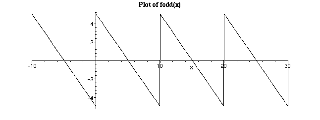
The Fourier sine series converges to the 2L-periodic extension of the above graph. We next define the Fourier sine coefficients , which we denote in function notation as b(n).

> b := n -> (2/L)*(int(f(x)*sin(n*Pi*x/L),x=0..L));

The above integral has not yet been evaluated. In this case Maple can evaluate these integrals exactly for particular values of n using the following function syntax.

> b(1);b(2);b(3);b(n);

Notice that the expressions for b(1), b(2), and b(3) are simplified, but the expression for b(n) is not. The and terms are not simplified because Maple does not know that n is an integer. However, b(n) can be simplified by substituting the known values for these trigonometric function.

> subs({sin(n*Pi)=0,cos(n*Pi)=(-1)^n},b(n));

> factor(%);

For more difficult problems where the integrals cannot be evaluated exactly, they can usually be evaluated numerically using the evalf command. In this case one should also replace int by Int in the expression defining the function b so that Maple does not try to symbolically evaluate the integral.

> evalf(b(2));evalf(b(4));

Next, we calculate and plot some partial sums. The partial sum for n = 1,2,...,N is a function of N and x.

> FSS := (N,x) -> sum(b(n)*sin(n*Pi*x/L),n=1..N);

If f(x) were a function that Maple could not evaluate the integrals in b(n) exactly, then the sum(...) in the above command should be replaced by evalf(sum(...)). Let us plot this sum for N=5 and N=20 and also plot fodd on the same axes.

> O2 := plot(FSS(5,x),x=-L..3*L,color=blue):

> O3 := plot(FSS(20,x),x=-L..3*L,color=magenta):

> plots[display]({O1,O2,O3}, title=`Plot of N=5 and N=20 Approximations to fodd(x)`, axesfont=[HELVETICA,BOLD,8], titlefont=[TIMES,BOLD,12], labels=[x,y], labelfont=[TIMES,BOLD,12]);

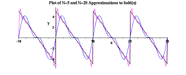
Observe the overshoot of the N=5 curve near x=2 and the overshoot of the N=20 curve near x=0.5. This illustrates the Gibbs phenomenon, and it can be shown that the maximum value of the overshoot is approximately 9% for all N.

We now repeat the above steps for feven, the even periodic extension of f(x).

> feven := x -> f(-x)*(H(x+L)-H(x)) + f(x)*(H(x)-H(x-L)) + f(-(x-2*L))*(H(x-L)-H(x-2*L)) + f(x-2*L)*(H(x-2*L)-H(x-3*L));

> E1 := plot(feven(x),x=-L..3*L,color=black):

> plots[display](E1, title=`Plot of feven(x)`, titlefont=[TIMES,BOLD,12]);

> a := n -> (2/L)*(int(f(x)*cos(n*Pi*x/L),x=0..L));

> a(0);a(1);a(n);

> subs({sin(n*Pi)=0,cos(n*Pi)=(-1)^n},a(n));

> factor(%);

> evalf(a(1));evalf(a(3));

> FCS := (N,x) -> a(0)/2 + sum(a(n)*cos(n*Pi*x/L),n=1..N);

> E2 := plot(FCS(5,x),x=-L..3*L,color=blue):

> E3 := plot(FCS(20,x),x=-L..3*L,color=magenta):

> plots[display]({E1,E2,E3}, title=`Plot of N=5 and N=20 Approximations to feven(x)`, axesfont=[HELVETICA,BOLD,8], titlefont=[TIMES,BOLD,12], labels=[x,y], labelfont=[TIMES,BOLD,12]);

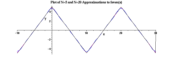
Clearly the convergence of the Fourier cosine series is better than that of the Fourier sine series. This is expected because the even periodic extension of f(x) is continuous whereas the odd periodic extension of f(x) has jump discontinuities at x = kL, for all integers k.

Variables Separable Partial Differential Equations

Let us illustrate the use of Fourier series for solving variables separable partial differential equations by considering the problem of heat conduction in a one-dimensional rod.

Example 2.

Consider the following initial boundary value problem.

, 0 < x < L, t > 0

u(0,t) = 0, u(L,t) = 0, t > 0

u(x,0) = f(x), 0 < x < L

The solution is known by separation of variables to be

,

where b(n) are the Fourier sine coefficients. Let f(x) = L/2 - x, for x in the interval [0,L], with L = 10, and take the thermal diffusivity constant k = 0.5. Approximate the solution u(x,t) at a few values of x and t and plot u as a function of (x,t). Animate the plot of the Nth partial sum approximations of u(x,t) for N = 2,4,...,20.

We define the constant k.

> k := 0.5;

The function f(x) and the constant L have already been defined in Example 1. In the following we will use the notation k, f(x), and L, so that the program can be easily modified by simply changing these definitions. However, if the boundary conditions are modified, then the infinite series solution for u(x,t) must be derived by separation of variables and entered. Let us define approximations u(N,x,t) to u(x,t) for N = 1,2,... by taking Nth partial sums.

> u := (N,x,t) -> sum(b(n)*sin(n*Pi*x/L)*exp(-k*t*(n*Pi/L)^2),n=1..N);

Since the Fourier integrals for b(n) can be evaluated symbolically for this function f(x), the value of the function u can be obtained simply by evaluating it at a particular value of (N,x,t). For example,

> u(20,L/4,0);u(20,L/4,5);u(20,L/4,10);

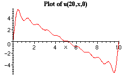
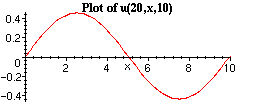
Let us plot the temperature profile as a function of x for t = 0 and t = 10 using N = 20 terms in the series.

> plot(u(20,x,0),x=0..L, title=`Plot of u(20,x,0)`, titlefont=[TIMES,BOLD,10]);

> plot(u(20,x,10),x=0..L, title=`Plot of u(20,x,10)`, titlefont=[TIMES,BOLD,10]);

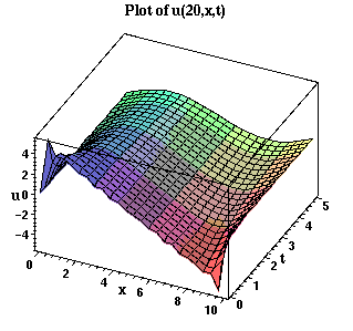
The evolution in time can be better visualized by making a 3-dimensional plot of u as a function of both x and t. Here we plot for x in [0,L] and t in [0,5].

> plot3d(u(20,x,t),x=0..L,t=0..5, style=PATCH, axes=BOXED, orientation=[-65,45], title=`Plot of u(20,x,t)`, axesfont=[HELVETICA,BOLD,8], titlefont=[TIMES,BOLD,12], labels=[x,t,u], labelfont=[TIMES,BOLD,12]);

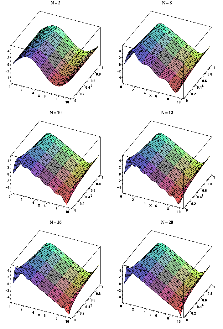
We have chosen a view orientation of so that we can see the t = 0 side of the plot. However, you can click the cursor on the plot which brings up a graphics context bar where you can rotate the plot to any view angle by changing the orientation. The convergence as the number N of terms increases can be dramatically demonstrated by animating the plot. Since b(n) = 0 for n an odd integer, the sum in u(20,x,t) contains 10 nonzero terms. In the following commands we make 10 frames corresponding to N = 2,4,...,20, and we plot for x in [0,L] and t in [0,1].

> Nseq := [seq(2*i,i=1..10)];

> A := seq(plot3d(u(N,x,t), x=0..L,t=0..1, title=`N = `.N), N=Nseq):

> plots[display](A, insequence=true, style=PATCH, axes=BOXED, orientation=[-65,45], axesfont=[HELVETICA,BOLD,8], titlefont=[TIMES,BOLD,12], labels=[x,t,u], labelfont=[TIMES,BOLD,12]);

In order to see the "movie," click the cursor on the plot which will bring up the animation context bar with buttons somewhat like those on a VCR. To the right of the orientation are the stop and play buttons. Click on play and you should see the animation. Observe that the slowest convergence as N increases is near t = 0 and the 9% overshoots in the Gibbs phenomenom move closer to the ends of the interval [0,L] as N increases.