Finite difference approximations

In this section we will learn how to approximate the derivatives of a differentiable function \(u = u(x)\) with respect to \(x\), where \(x \in [X_L,X_R]\).

Finite differencing on uniform grids

Suppose we want to approximate the second derivative \(\frac{\partial^2 u(x)}{\partial x^2}\). For the approximation of first derivative \(\frac{\partial u(x)}{\partial x}\) see the examples below.

First, we need to choose where (i.e. “for what values of \(x \in [X_L,X_R]\)“) we would like to know the approximate value of the derivative \(\frac{\partial^2 u(x)}{\partial x^2}\). A natural choice is at a set of \(n+1\) grid points on a equidistant grid

\begin{equation} x_i = X_L + i h, \qquad i = 0,\ldots,n, \qquad h = \frac{X_R-X_L}{n}. \end{equation}

Here \(h\) is the grid spacing (known as grid length or grid size) which has been chosen such that \(x_0 = X_L\) and \(x_n = X_R\).

Next, in order to find an approximation to the second derivative we expand the solution in a Taylor series around \(x\) (at \(x+h\) and \(x-h\)):

\begin{eqnarray} u(x+h) = u(x) + h \frac{\partial u(x)}{\partial x} + h^2/2 \frac{\partial^2 u(x)}{\partial x^2} + h^3/6 \frac{\partial^3 u(x)}{\partial x^3} + h^4/24 \frac{\partial^4 u(x)}{\partial x^4} + \mathcal{O}(h^5), \\ u(x-h) = u(x) - h \frac{\partial u(x)}{\partial x} + h^2/2 \frac{\partial^2 u(x)}{\partial x^2} - h^3/6 \frac{\partial^3 u(x)}{\partial x^3} + h^4/24 \frac{\partial^4 u(x)}{\partial x^4} + \mathcal{O}(h^5). \end{eqnarray}

Adding these equations together we get:

\begin{equation} u(x+h) + u(x-h) = 2 u(x) + h^2 \frac{\partial^2 u(x)}{\partial x^2} + h^4/12 \frac{\partial^4 u(x)}{\partial x^4} + \mathcal{O}(h^5), \end{equation}

which can be rearranged to

\begin{equation} \frac{u(x+h) -2 u(x) + u(x-h)}{h^2} - \frac{\partial^2 u(x)}{\partial x^2} = h^2/12 \frac{\partial^4 u(x)}{\partial x^4} + \mathcal{O}(h^3). \end{equation}

We therefore obtain

\begin{equation} \frac{\partial^2 u(x)}{\partial x^2} = \frac{u(x+h) -2 u(x) + u(x-h)}{h^2} + \mathcal{O}(h^2). \end{equation}

The quotient on the right hand side is thus a second order accurate approximation to \(\frac{\partial^2 u(x)}{\partial x^2}\). In particular we see that if we choose \(x=x_i\) and use the fact that \(x_i \pm h = x_{i \pm 1}\) and also introduce the notation \(u_i = u(x_i)\) we may write:

\begin{equation} \frac{\partial^2 u_i}{\partial x^2} = \frac{\partial^2 u(x_i)}{\partial x^2} \approx \frac{u(x_{i+1}) -2 u(x_i) + u(x_{i-1})}{h^2} = \frac{u_{i+1} -2 u_i + u_{i-1}}{h^2}. \end{equation}

This is called a central three-point finite difference approximation for the second derivative.

Biased stencils

Assuming that we know \(u_i, \, i = 0,\ldots,n\), we see that it is not possible to use the above centeral finite difference stencil at the boundary points \(x_0\) and \(x_n\). Using the central stencil at the end points would require knowing the solution \(u\) at \(x_{-1}\) and \(x_{n+1}\) which are outside the domain. Instead we can derive biased (or one-sided) stencils at the end points of the grid. We again use Taylor’s theorem, but now we expand in Taylor series the interior solutions around end points. Expanding the interior solutions \(u_1\) and \(u_2\) around the left end-point \(x_0\), we obtain:

\begin{eqnarray} u_1 = u_0 + h \frac{\partial u_0}{\partial x} + h^2/2 \frac{\partial^2 u_0}{\partial x^2} + h^3/6 \frac{\partial^3 u_0}{\partial x^3} + h^4/24 \frac{\partial^4 u_0}{\partial x^4} + \mathcal{O}(h^5), \\ u_2 = u_0 + 2h \frac{\partial u_0}{\partial x} + 4h^2/2 \frac{\partial^2 u_0}{\partial x^2} + 8h^3/6 \frac{\partial^3 u_0}{\partial x^3} + 16h^4/24 \frac{\partial^4 u_0}{\partial x^4} + \mathcal{O}(h^5). \end{eqnarray}

Now we can subtract two times the first equation form the second equation yielding the first order accurate approximation

\begin{equation} \frac{u_2 - 2u_1 + u_0}{h^2} = \frac{\partial^2 u_0}{\partial x^2} + \mathcal{O}(h). \end{equation}

If we also include the expansion for \(u_3\) we can get the second order approximation

\begin{equation} \frac{-u_3 + 4u_2 - 5u_1 + 2u_0}{h^2} = \frac{\partial^2 u_0}{\partial x^2} + \mathcal{O}(h^2). \end{equation}

To check the coefficients of the stencils we can consider the special cases of a constant and a linear function which should be differentiated exactly by a first and second order accurate method respectively. Obviously both stencils are exact for a constant function \(u(x) = c\) (the coefficients add up to zero). Additionally the second approximation is exact for the linear function \(u(x)=x\) on the grid \(x_0 = 0, x_1 = 1, x_2 = 2, x_3 = 3\) with \(h=1\). The second derivative of a linear is zero which is exactly what comes out, i.e. \(-3 + 2\times 4 - 5\times 1 + 1\times 0 = 0\).

Similarly, we can obtain the second order finite difference approximation for the second derivative at the right end-point:

\begin{equation} \frac{-u_{n-3} + 4u_{n-2} - 5u_{n-1} + 2u_n}{h^2} = \frac{\partial^2 u_n}{\partial x^2} + \mathcal{O}(h^2). \end{equation}

Higher order approximations

The above procedure can in principle be extended to use more points on the grid (instead of only 3 or 4 points), yielding higher order accurate approximations (higher than second-order accuracy). For a good list of stencil weights see here. A general algorithm for finding finite difference stencils of all orders has been found by Bengt Fornberg and is described in his excellent review paper.

In what follows we discus how the above approximations can be implemented in Fortan.

Finite difference examples in Fortran

This section discusses implementations of the finite difference approximations discussed above. The Fortran codes for the following examples can be found in the course repository in directory “Labs/lab3”.

Here we only consider the approximation of the first-order derivative. Higher order derivatives can be computed similarly. We present three examples. In the first example we approximate the derivative using a three point second order accurate stencil on an equidistant grid. In the second example we use Bengt Fornberg’s subroutine Fornberg_weights.f90 to find the stencil that extends over all grid-points. This would, in principle, give an approximation of maximal order. However, we will find that this approach does not work well on equidistant grids. In the third example we investigate the performance of the maximal-order finite difference stencil (usually called spectral finite differences) on graded Legendre-Gauss-Lobatto grids. Recall that we have already discussed such grids in Homework 3 in the context of numerical integration.

Example 1: a low-order finite difference method

Consider the function \(f(x) = e^{ \cos (\pi x)}\) and its first derivative \(f'(x) = -\pi \sin (\pi x) e^{\cos (\pi x)}\) where \(x\in[-1,1]\). We further consider the equidistant grid

\begin{equation} x_i = -1 + i h, \qquad i = 0,\ldots,n, \qquad h = \frac{2}{n}, \end{equation}

and use Taylor series (similar to what we did above) to approximate the first derivative of \(f\) at \(x_i\), i.e. \(f'(x_i)\), denoted by \((f')_i\):

\begin{eqnarray} (f')_i = \left\{ \begin{array}{ll} \frac{-1.5 f_{i}+2f_{i+1}-0.5 f_{i+2}}{h} & i = 0\\ \frac{0.5 f_{i+1}- 0.5 f_{i-1}}{h} & i = 1,\ldots,n-1\\ \frac{1.5 f_{i}-2f_{i-1} + 0.5 f_{i-2}}{h} & i = n \end{array} \right. \end{eqnarray}

Since we know the exact value of the derivative, we can compute the exact error in our finite difference approximation. Hence, using a decreasing sequence of \(h\) values, we can easily check if the error decreases as we expect. We notice that since we will have different number of grid-points for different \(h\) values, we declare the array x to be a 1D allocatable array. We also declare the arrays holding the function, the approximation to the derivative, and the exact derivative as allocatable (see line 6). The finite difference stencils on the other hand will be the same independent of the number of grid points and can thus be stored in a fixed size array diff_weights(1:3,1:3). Recall that in Fortran the default indexation starts with one, and hence an equivalent declaration would be diff_weights(3,3).

The code loops over all \(n=4,5,\ldots,100\) and allocates arrays of size \(n+1\) (line 10), computes the grid spacing, the grid, the function, and the exact derivative (lines 12-18). We then set up the array that holds the finite difference weights (note that due to the \(h\) dependency of the weights, we have to change the weights for every loop) and compute the finite difference approximation to \(f'(x)\) (lines 23-45). Finally, on line 46 we compute the maximum error on the grid and print it to screen.

program differentiate1
  implicit none
  real(kind = 8), parameter :: pi = acos(-1.d0)
  integer :: n,i,j
  real(kind = 8) :: h,diff_weights(1:3,1:3)
  real(kind = 8), dimension(:), allocatable :: x,f,df,df_exact

  do n  = 4,100
     ! Allocate memory for the various arrays
     allocate(x(0:n),f(0:n),df(0:n),df_exact(0:n))
     ! Set up the grid.
     h = 2.d0/dble(n)
     do i = 0,n
        x(i) = -1.d0+dble(i)*h
     end do
     ! The function and the exact derivative
     f = exp(cos(pi*x))
     df_exact = -pi*sin(pi*x)*exp(cos(pi*x))

     ! Set up weights for a finite difference stencil
     ! using three gridpoints
     ! In the interior we use a centered stencil
     diff_weights(1:3,1) = (/-0.5d0,0.d0,0.5d0/)
     ! To the left we use a biased stencil
     diff_weights(1:3,2) = (/-1.5d0,2.d0,-0.5d0/)
     ! To the right we use a biased stencil
     diff_weights(1:3,3) = (/1.5d0,-2.d0,0.5d0/)
     ! scale by 1/h
     diff_weights = diff_weights/h

     ! Now differentiate
     ! To the left is a special case
     df(0) = 0.d0
     do j = 1,3
        df(0) = df(0) + diff_weights(j,2)*f(j-1)
     end do
     ! Now interior points
     do i = 1,n-1
        df(i) = sum(diff_weights(1:3,1)*f((i-1):(i+1)))
     end do
     ! Finally, special case to the right
     df(n) = 0.d0
     do j = 1,3
        df(n) = df(n) + diff_weights(j,3)*f(n-(j-1))
     end do
     write(*,'(I3,2(ES12.4))') n,h,maxval(abs(df-df_exact))

     ! Deallocate the arrays
     deallocate(x,f,df,df_exact)
  end do

end program differentiate1

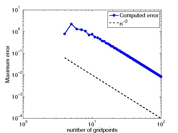
The results from the output of the above program is displayed in the figure below. As we see the slope of the error is the same as a \(h^{2} \sim n^{-2}\) indicating that the implementation may be correct (confirming that convergence is second order).

Example 2: maximum order on an equidistant grid

Next, we use a finite difference stencil that extends over all \(n+1\) grid-points to approximate the first derivative of \(f\). The weights of the stencil are computed by Bengt Fornberg’s weights subroutine Fornberg_weights.f90, which is located in the course repository in directory “Labs/lab3”.

! This program differentiates functions (up to m-th derivative)
! using a finite difference stencil with maximum width
! computed by Bengt Fornberg's weights subroutine (Fornberg_weights.f90)
! on an equidistant grid

program differentiate2
  implicit none
  real(kind = 8), parameter :: pi = acos(-1.d0)
  integer :: n,i,j,m
  real(kind = 8) :: h,z
  real(kind = 8), dimension(:), allocatable :: x,f,df,df_exact
  real(kind = 8), dimension(:,:), allocatable :: c

  m = 1  !the highest derivative (here 1)
  do n  = 4,100
     ! Allocate memory for various arrays
     allocate(x(0:n),f(0:n),df(0:n),df_exact(0:n))
     allocate(c(0:n,0:m))
     ! Set up the grid.
     h = 2.d0/dble(n)
     do i = 0,n
        x(i) = -1.d0+dble(i)*h
     end do
     ! The function and the exact derivative
     f = exp(cos(pi*x))
     df_exact = -pi*sin(pi*x)*exp(cos(pi*x))
     ! Find the difference stencil that uses all grid points
     do i = 0,n
        df(i) = 0.d0
        z = x(i)
        call Fornberg_weights(z,x,n,m,c)
        do j = 0,n
           df(i) = df(i) + c(j,1)*f(j)
        end do
     end do
     write(*,'(ES12.4)') maxval(abs(df-df_exact))
     ! Deallocate the arrays
     deallocate(x,f,df,df_exact,c)
  end do
end program differentiate2

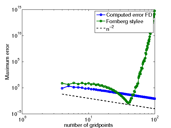
The results from the output of the above program is displayed in the figure below, together with the results obtained from the first example. We observe that for small number of grid points, the wide stencil may deliver better results, compared to the three-point stencil. However, for large number of grid points, wide stencils have poor performance.

Example 3: maximum order on a Legendre-Gauss-Lobatto grid

Finaly, we use Bengt Fornberg’s wide stencil on a Legendre-Gauss-Lobatto grid.

! This program differentiates functions (up to m-th derivative)
! using a finite difference stencil with maximum width
! computed by Bengt Fornberg's weights subroutine (Fornberg_weights.f90)
! on a Legendre-Gauss-Lobatto grid computed by the subroutine lglnodes.f90

program differentiate3
  implicit none
  real(kind = 8), parameter :: pi = acos(-1.d0)
  integer :: n,i,j,m
  real(kind = 8) :: z
  real(kind = 8), dimension(:), allocatable :: x,f,df,df_exact,w
  real(kind = 8), dimension(:,:), allocatable :: c

  m = 1  !the highest derivative (here 1)
  do n  = 4,100
     ! Allocate memory for various arrays
     allocate(x(0:n),f(0:n),df(0:n),df_exact(0:n),w(0:n))
     allocate(c(0:n,0:m))
     ! Set up the grid.
     call lglnodes(x,w,n)
     ! The function and the exact derivative
     f = exp(cos(pi*x))
     df_exact = -pi*sin(pi*x)*exp(cos(pi*x))
     ! Find the difference stencil that uses all grid points
     do i = 0,n
        df(i) = 0.d0
        z = x(i)
        call Fornberg_weights(z,x,n,m,c)
        do j = 0,n
           df(i) = df(i) + c(j,1)*f(j)
        end do
     end do
     write(*,'(ES12.4)') maxval(abs(df-df_exact))
     ! Deallocate the arrays
     deallocate(x,f,df,df_exact,c,w)
  end do
end program differentiate3

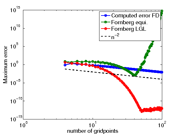
The results from the output of the above program is displayed in the figure below, together with the results obtained from the first two examples. We observe that the wide stencil has an excellent performance on LGL nodes, as it does not suffer from roundoff due to ill-conditioning that occur on equidistant grids. In general, LGL nodes deliver much better grid distributions than uniform distributions.