Homework 3
Due extended to 23.59, Sep/30/2020 (Original due Sep/27/2020)
Fortran and numerical integration (quadrature)
Consider the integral
with \(k = \pi\) or \(\pi^2\). In this homework you will experiment with two different ways of computing approximate values of \(I\). After doing this homework you will have written a Fortran program from scratch, called a subroutine that someone else has written and gained some knowledge of the accuracy of some different methods for numerical integration (quadrature). In future homework we will see how these computations can be performed in parallel.
I will talk about the most basic quadrature rules in class. For a more detailed description you can refer to my lecture notes.
Part I: Trapezoidal rule
The trapezoidal rule belongs to a class of Newton-Cotes quadrature rules that approximate integrals using equidistant grids. The order of a composite Newton-Cotes method is typically \(s\) or \(s+1\), where \(s\) is the number of points in each panel (2 for the Trapezoidal rule).
For a set of equi-distant grid points \(x_i = X_L + ih, \ \ i = 0,\ldots,n, \ \ h = \frac{X_R-X_L}{n}\) on the interval \([X_L, X_R]\), the composite trapezoidal rule reads:
Write a Fortran program that uses the composite trapezoidal rule to approximate the above integral for both \(k = \pi\) and \(k=\pi^2\) and for \(n = 2,3,\ldots,N\), where you should pick \(N\) so that the absolute error is smaller than \(10^{-10}\). Note that here \(X_L = -1\) and \(X_R = 1\).
- In your report, plot the error against \(n\) using a logarithmic scale for both axes.
- Can you read off the order of the method from the slopes? How does this agree with theory?
- What is special with the integrand in the case \(k = \pi\) and why does it make the method converge faster than expected? For a careful study of the superior performance of the trapezoidal rule on special functions take a look at the Euler-Maclaurin formula.
Part II: Gauss Quadrature
In Newton–Cotes quadrature rules, it is assumed that the value of the integrand is known at equally spaced points. If it is possible to change the points at which the integrand is evaluated, other methods such as Gauss quadrature and Clenshaw–Curtis quadrature are often more suitable.
In Gauss quadrature the location of the grid-points \(z_i\) (usually referred to as quadrature nodes) and the quadrature weights \(\omega_i\) are chosen so that the order of the approximation to the weighted integral
is maximized, where the weight function \(w(z)\) is assumed to be positive and
integrable (in this homework \(w(z) = 1\)). Such “optimal” nodes turn out to be the roots of orthogonal polynomials associated with the weight function
\(w(z)\). For the case \(w(z) = 1\), we use Legendre polynomials and obtain the weights and nodes by a call to the subroutine lglnodes.f90 (which is a Fortran version of Greg von Winckel’s matlab version). Use the subroutine lglnodes.f90 from the course repository and compute the integral by the following code that implements the above formula:
call lglnodes(x,w,n)
f = exp(cos(pi*pi*x))
Integral_value = sum(f*w)
Again:
- plot the error against \(n\) using a logarithmic scale for both axes (perhaps in the same figure).
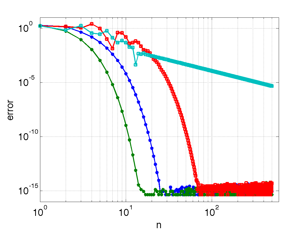
- For Gauss quadrature the error is expected to decrease as \(\varepsilon(n) \sim C^{-\alpha n}\). Try some different \(C\) and \(\alpha\) to see if you can fit the computed error curves.
A few notes
- The errors should look something like the figure below (note that you should label the curves, I left them out on purpose).
For this homework you will call a routine from another file which means that to build your executable you will have to compile two object files and then link them together:
$ gfortran -O3 -c gq_test.f90
$ gfortran -O3 -c lglnodes.f90
$ gfortran  -o gq_test.x  gq_test.o lglnodes.o
A better way of doing this is to use a makefile. I will talk about this in class. See also the Makefile section.
It is probably a good idea to use allocatable arrays for
x,w,faboveallocate(x(0:n),f(0:n),w(0:n)) ...Code here... deallocate(x,f,w)as their size will change as you change \(n\). Don’t forget to deallocate the arrays.
Do not forget to update the top-level README file in your repository. You will also need to include a low-level README file in your HW3 subdirectory.
Write up your findings neatly as a report and check it in to your repository. In general you should start your report with a brief description of the problem and continue with the procedure that you carry out and the methods that you use to solve the problem and obtain results. You then present your results (which can be in form of tables and/or figures, etc.) and discuss/analyze them. Finally you finish your report with your conclusions. Choose appropriate names for different sections of your report.