Homework 4

Due extended to 23.59, Oct/16/2020 (Original due Oct/11/2020)

Curvilinear coordinates

In this homework you will compute derivatives and integrals on a logically rectangular domain (i.e. it has four sides and no holes), denoted by \(\Omega\). The main strategy is to use a smooth mapping \((x,y)=(x(r,s),y(r,s))\) from a reference element \(\Omega_{\text{R}} = \{(r,s) \in [-1,1]^2\}\) to \(\Omega\). This allows us to transfer the computations from \(\Omega\) to \(\Omega_{\text{R}}\).

I. Differentiation on \(\Omega\)

Let \(u = u(x,y)\) be a continuously differentiable function of \(x\) and \(y\), where \((x,y) \in \Omega\). We want to approximate the partial derivative of \(u\) with respect to \(x\) and \(y\). We first consider \(x=x(r,s)\) and \(y=y(r,s)\) as functions of \(r\) and \(s\), where \((r,s) \in \Omega_{\text{R}} = [-1,1]^2\). We then use the chain rule and write

\begin{equation*} \frac{\partial u}{\partial x} = \frac{\partial u}{\partial r} \frac{\partial r}{\partial x}+\frac{\partial u}{\partial s} \frac{\partial s}{\partial x}, \qquad \text{alternative notation:} \quad u_x = u_r \, r_x + u_s \, s_x \end{equation*}

\begin{equation*} \frac{\partial u}{\partial y} = \frac{\partial u}{\partial r} \frac{\partial r}{\partial y}+\frac{\partial u}{\partial s} \frac{\partial s}{\partial y}, \qquad \text{alternative notation:} \quad u_y = u_r \, r_y + u_s \, s_y \end{equation*}

We next introduce a Cartesian grid on the reference element \(\Omega_{\text{R}} = [-1,1]^2\):

hr = 2.d0/dble(nr)
hs = 2.d0/dble(ns)
do i = 0,nr
   r(i) = -1.d0 + dble(i)*hr
end do
do i = 0,ns
   s(i) = -1.d0 + dble(i)*hs
end do

and compute \(u_r\) and \(u_s\) by standard finite difference formulas (see the subroutine differentiate). It is left to find \(r_x, r_y, s_x, s_y\). For this, we can easily compute \(x_r, x_s, y_r, y_s\) and then use the above two formulas with \(u = x\) and \(u = y\). This gives

\begin{equation*} \left[ \begin{array}{cc} r_x & s_x \\ r_y & s_y \end{array} \right] \left[ \begin{array}{cc} x_r & y_r \\ x_s & y_s \end{array} \right] = \left[ \begin{array}{cc} 1 & 0 \\ 0 & 1 \end{array} \right] \qquad \Rightarrow \qquad \left[ \begin{array}{cc} r_x & s_x \\ r_y & s_y \end{array} \right] = \left[ \begin{array}{cc} x_r & y_r \\ x_s & y_s \end{array} \right]^{-1}. \end{equation*}

II. Integration on \(\Omega\)

It is also possible to compute integrals on logically rectangular domains. For example, we have:

\begin{equation*} \int_{\Omega} f(x,y) dxdy = \int_{-1}^1 \int_{-1}^1 f(x(r,s),y(r,s)) \, J(r,s) \, d r d s, \end{equation*}

where \(J(r,s) = x_r y_s - x_s y_r\) is the surface element. The second integrand can be approximated on the reference element, for example with the 2D trapezoidal rule.

Assignments:

0. Start with pulling the files residing in the course Bitbucket repository in “hw4” directory.

1. Make and run the program homework4.f90 and use the Matlab script (or some other plotting tool) to display the grid.

2. Use the above matrix formula to find (compute numerically) \(r_x, r_y, s_x, s_y\).

3. Write a subroutine, say integral_omegaR.f90, that would numerically integrate any desired function (the integrand) on the reference element \(\Omega_{\text{R}} = [-1,1]^2\), for instance by the trapezoidal rule. Note that this will require a double integration and hence a slightly different procedure from the one-dimensional trapezoidal rule that you did in previous homework. Before proceeding to next step, verify your code integral_omegaR.f90. One possibility to verify your code is to change the mapping in xycoord.f90 to map the reference element \(\Omega_{\text{R}}\) into some geometrical shape \(\Omega\) for which you know the area (for example a sector of an annulus), and check that your code correctly computes the area of \(\Omega\), e.g. by integrating a unit integrand \(u(x,y)=1\) on \(\Omega\). Do not forget to include the Jacobian in your integrand when you use integration over \(\Omega_{\text{R}}\) to compute an integral over \(\Omega\).

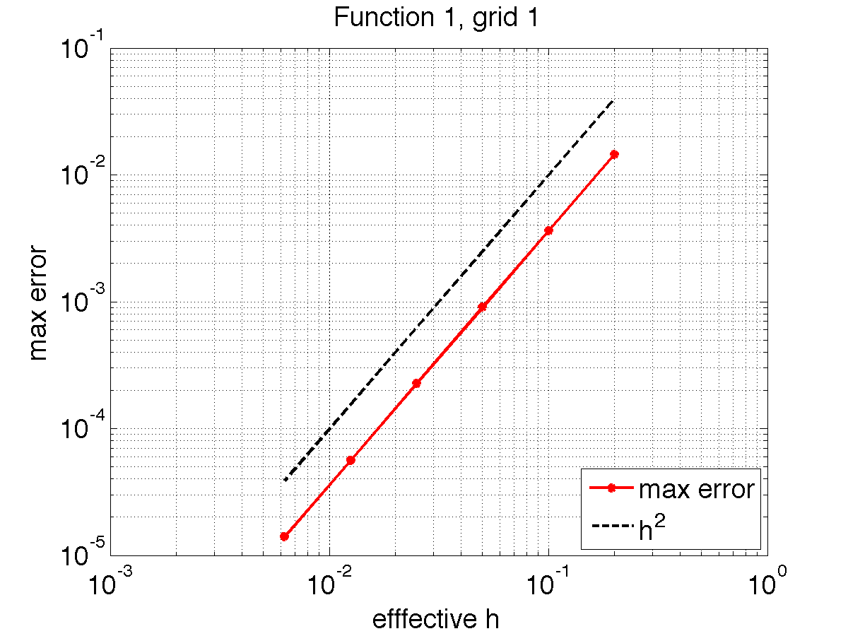
4. Compute \(u_x\) and \(u_y\) for some different functions \(u(x,y)\) and some different mappings. Using your quadrature subroutine integral_omegaR.f90 approximate the error

   \begin{equation*} e_2(h_r,h_s) = \left(\int_{\Omega} \left(u_x(x,y)+u_y(x,y) - \left[(u_{\rm exact})_x + (u_{\rm exact})_y \right] \right)^2 dxdy \right)^{1/2}, \end{equation*}

   and plot the error as a function of the grid spacing for the different functions and the different mappings.

5. Use the chain rule to find an expression for \(\Delta u = u_{xx}+u_{yy}\). Discretize it and repeat the experiments above.

6. Write up your findings neatly as a report and check it in to your repository. In general you should start your report with a brief description of the problem and continue with the procedure that you carry out and the methods that you use to solve the problem and obtain results. You then present your results (which can be in form of tables and/or figures, etc.) and discuss/analyze them. Finally you finish your report with your conclusions. Choose appropriate names for different sections of your report.

Sample results

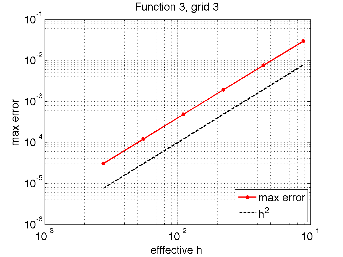
Below you find some sample results. Note that the errors are messured in the max-norm so the results you produce are not going to be identical with mine. Also note that the errors are plotted as a function of an effective gridsize \(h_{\rm eff} = \sqrt{h_r h_s \max J}\). Here we use 3 combinations of grids and functions:

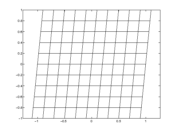
The three combinations are

! Combination 1
x_coord = r+0.1d0*s
y_coord = s
u = sin(xc)*cos(yc)

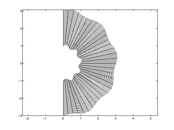
! Combination 2
x_coord = (2.d0+r+0.1d0*sin(5.d0*pi*s))*cos(0.5d0*pi*s)
y_coord = (2.d0+r+0.1d0*sin(5.d0*pi*s))*sin(0.5d0*pi*s)
u = exp(xc+yc)

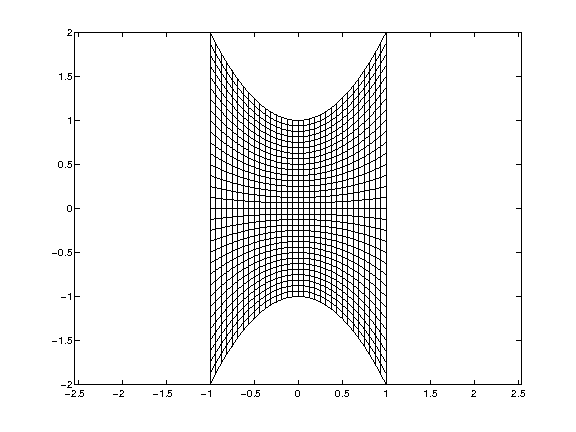
! Combination 3
x_coord = r
y_coord = s + s*r**2
u = xc**2+yc**2

And the grids and results are: