Partial differential equations
I. Initial-boundary value problems
Partial differential equations (PDEs) are important mathematical models that describe many physical systems in science and engineering. They are used to predict a wide range of phenomena in the past and future, from climate changes, to the growth of cancerous tumors, to the spread of epidemics, to economic crises, to the location of earthquakes, to the existance of black holes, etc.
As an example, wave equarion is a PDE used to model the propagation of waves in a medium (such as seismic waves in the Earth, electromagnetic waves in the air, sound waves in the ocean, and gravitational waves in the universe). In a non-homogeneous two-dimensional medium (denoted by \(D \subset {\mathbb R}^2\)), where the wave speed is not constant, the wave equation in the conservative form reads:
The solution \(u = u(x,y,t)\) to the wave equation is a function of space (\(x,y\)) and time (\(t\)) and may represent the displacement in a solid, sound pressure, particle velocity, or, under certain conditions, the electric or magnetic fields. The quantity \(a\) is the “wave speed” in the medium. Here the divergence \(\nabla \cdot\) and gradient \(\nabla\) are partial differential operators with respect to spatial variables \((x,y)\), and \(u_{tt}\) is the second partial derivative of \(u\) with respect to time \(t\).
The above equation is in (2+1) dimensions: 2 spatial dimensions and 1 temporal dimension, referred to as 2D wave equation. We need to augment the PDE with two initial conditions (at \(t = 0\)) and boundary conditions (at the boundary of the domain, denoted by \(\partial D\)):
In general, a partial differential equation (e.g. wave equation) together with its corresponding intial and boundary conditions is called an initial-boundary value problem.
II. Numerical solutions to initial-boundary value problems
Many real-world problems cannot be solved by traditional experimental or theoretical tools, either because it is impossible (e.g. prediction of climate change), or because it is too expensive or time-consuming (e.g. determination of structure of proteins), or because experimentation is dangerous (e.g. study of toxic materials and explosions). As the third pillar of science, scientific computing tries to model complex scientific problems by PDEs and numerically solve them using computers. A major task of scientific computing is therefore to approximate the solution to PDEs, with high accuracy and efficiency.
As computers have finite amount of memory we will have to restrict ourselves to finding approximate solutions to the wave equation at a finite number of \((x,y) \in D\) and \(t \in [0, T]\) values. One approach to do this is called finite difference approximation. There are many other approaches such as the finite element method, fininte volume method, and spectral method. Here we focus on the finite difference method.
Method of lineas and finite differencing on uniform grids
The method of lines (MOL) is a popular technique for solving time-dependent PDEs. It consists of two steps:
- First, the PDE problem is discretized in the spatial domain \(D\) into \(N\) grid proint to obtain a semi-discrete problem leaving the time continuous. This gives us a system of \(N\) ODEs in time.
- The semi-discrete problem (i.e. the system of ODEs) is then discretized in time to obtain a fully descrete solution in both space and time.
Let \(D = [-1,1]^2\) be a rectangular spatial domain. We uniformly discretize \(D\) into a uniform grid with \(n_x\) grid points in the \(x\) direction and \(n_y\) grid points in the \(y\) direction:
Here \(h_x\) and \(h_y\) are the grid spacing (known as grid length or grid size) in the \(x\) and \(y\) directions, respectively. In total we will have \(N = n_x \, n_y\) grid ponits.
Let \(u_{i,j}(t)\) denote the semi-discrete approximation for the exact value of the semi-descrete solution \(u(x_i,y_j,t)\), that is, let
Moreover, let
be the Laplacian. Recall that \(\nabla \cdot \left( a(x,y) \, \nabla u \right) = (a \,u_x)_x + (a \,u_y)_y\). We employ the following second-order accurate centered finite difference scheme for approximating the Laplacian:
\begin{eqnarray} &(a(x_i,y_j) \, u_x(x_i,y_j,t))_x \approx & D_-^x\left(E^x(a_{i,j}) \, D_+^x u_{i,j}(t) \right), \\ &(a(x_i,y_j) \, u_y(x_i,y_j,t))_y \approx & D_-^y\left(E^y(a_{i,j}) \, D_+^y u_{i,j}(t) \right), \end{eqnarray}
where
\begin{eqnarray} D_+^x u_{i,j} = \frac{u_{i+1,j}-u_{i,j}}{h_x}, \ \ D_-^x u_{i,j} = \frac{u_{i,j}-u_{i-1,j}}{h_x}, \ \ E^x(a_{i,j}) = \frac{a_{i,j} + a_{i+1,j}}{2},\\ D_+^y u_{i,j} = \frac{u_{i,j+1}-u_{i,j}}{h_y}, \ \ D_-^y u_{i,j} = \frac{u_{i,j}-u_{i,j-1}}{h_y}, \ \ E^y(a_{i,j}) = \frac{a_{i,j} + a_{i,j+1}}{2}. \end{eqnarray}
This gives:
\begin{eqnarray} D_-^x\left(E^x(a_{i,j}) D_+^x u_{i,j}(t)\right) = \frac{(a_{i+1,j}+a_{i,j})}{2h_x^2}u_{i+1,j}(t) - \frac{(a_{i+1,j}+2a_{i,j}+a_{i-1,j})}{2h_x^2}u_{i,j}(t) + \frac{(a_{i,j}+a_{i-1,j})}{2h_x^2}u_{i-1,j}(t), \\ D_-^y\left(E^y(a_{i,j}) D_+^y u_{i,j}(t)\right) = \frac{(a_{i,j+1}+a_{i,j})}{2h_y^2}u_{i,j+1}(t) - \frac{(a_{i,j+1}+2a_{i,j}+a_{i,j-1})}{2h_y^2}u_{i,j}(t) + \frac{(a_{i,j}+a_{i,j-1})}{2h_y^2}u_{i,j-1}(t). \end{eqnarray}
Hence we obtain a 5-point stencil that is a second-order accurate approximation of the Laplacian:
\begin{eqnarray} L_{i,j}(t) = \alpha_{i,j}^L \, u_{i-1,j}(t) + \alpha_{i,j}^R \, u_{i+1,j}(t) + \alpha_{i,j}^B \, u_{i,j-1}(t) + \alpha_{i,j}^T \, u_{i,j+1}(t) + \alpha_{i,j}^C \, u_{i,j}(t), \end{eqnarray}
where the weights \(\alpha_{i,j}^L, \alpha_{i,j}^R, \dotsc\) are easily obtained in terms of the wave speed \(a\) and the grid sizes \(h_x, h_y\).
Now if we let \(f_{i,j}(t) = f(x_i,y_j,t)\), we arrive at a set of \(n_x \, n_y\) ODEs in time:
We finally discretize the time interval \([0,T]\) into \(n_t+1\) grid points with a time step \(\Delta t\):
Now let \(u_{i,j}^k \approx u_{i,j}(t_k)\) be the fully discrete approximation. We can solve this ODE system by a simple centered difference scheme:
\begin{equation} \frac{u_{i,j}^{k+1}-2 u_{i,j}^k+u_{i,j}^{k-1}}{(\Delta t)^2} = L_{i,j}^k + f_{i,j}^k, \end{equation}
which gives
\begin{equation} u_{i,j}^{k+1} = 2 u_{i,j}^k- u_{i,j}^{k-1} + (\Delta t)^2 \, (L_{i,j}^k + f_{i,j}^k), \qquad k=1, \dotsc, n_t-1. \end{equation}
This means to obtain the solution at \(t_{k+1}\), we will need the solution at two previous time steps, .i.e. at \(t_k\) and \(t_{k-1}\). We obtain the solution at the first two time steps, i.e. at \(t_0 =0\) and \(t_{1} = \Delta t\), by the two initial conditions as follows.
The first one is easy. We directly use the first initial condition \(u(x,y,0)=f_1(x,y)\):
The second one is more involved, and one should be careful so that the secon-order accuracy is preserved. First, recall that the second initial conditions is \(u_t(x,y,0) = f_2(x,y)\). We write the Taylor’s expnasion
We use the second initial condition to find \(u'_{i,j}(0)\) and use the PDE to find \(u''_{i,j}(0)\) in the right hand side of the above equation. We then obtain \(u_{i,j}^1\) in terms of \(u_{i,j}^0\):
This completes the numerical algorithm and delivers a second-order accurate method in both space and time.
III. Verification: convergence and manufactured solutions
Suppose that we would like to implement the above numerical method on a computer to solve a given initial-boundary value problem, such as the above wave propagation problem. How can we make sure that our code works correctly, that is, how can we make sure that our implemented numerical method correctly approximates the PDE problem? This is a crucial question in scientific computing, refered to as verification.
We will need to verify the convergence, that is, we need to verify that the approximate solution converges to the true solution with the advertized theoretical rate. For instance, let \(h=h_x=h_y\) and \(\Delta t = c \, h\), and consider the maximum error at a fixed time \(t_k\):
$$\varepsilon (h)= \max_{i,j} | u(x_i,y_j,t_k) - u_{i,j}^k |.$$
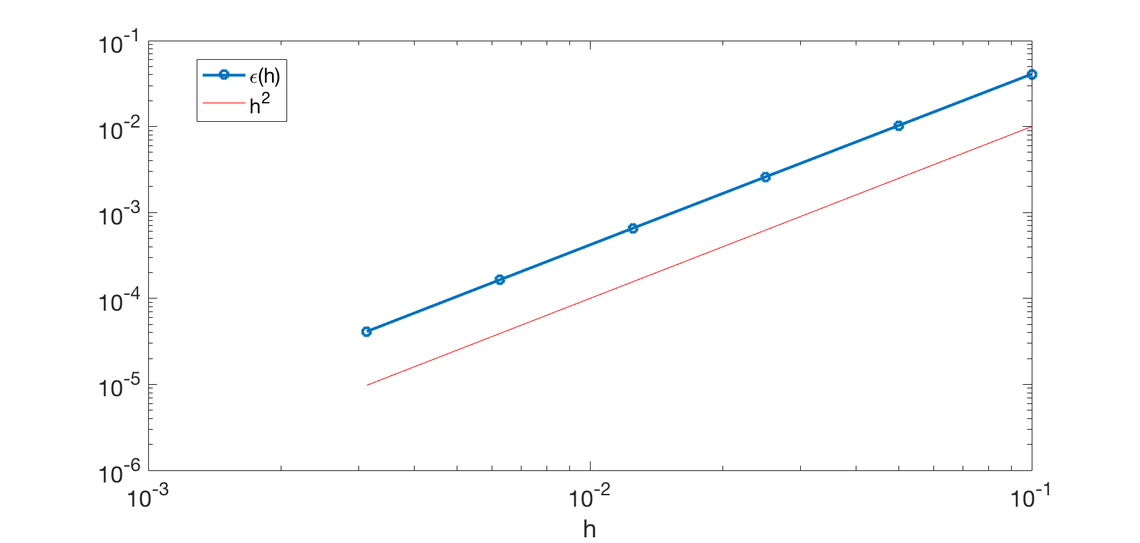
We want to make sure that \(\varepsilon(h) \sim \mathcal{O}(h^2)\). For this we will need to measure the error for various \(h\) values and verify that it is proportional to \(h^2\).
A major issue here is that the computation of \(\varepsilon\) requires the knowledge of the true solution \(u\) that is not available to us. This is where the method of manufactured solution comes in, as follows.
First we manufacture a solution for the PDE problem, e.g. a trigonometric function:
\begin{equation}\label{mms} u(x,y,t) = \sin(\omega t -k_x \, x) \, \sin(k_y \, y), \end{equation}
We then adjust the initial-boundary value problem so that this is indeed its solution. All we need to do is to plug this manufactured solution into the problem and obtain the forcing \(f(x,y,t)\), the initial data \(f_1(x,y)\) and \(f_2(x,y)\), and the boundary data \(g(x,y,t)\). For example, with \(u\) as above, we would get:
\begin{align*} & f(x,y,t)=(k_x^2 + k_y^2-\omega^2) \, \sin(\omega \, t -k_x \, x) \, \sin(k_y \, y),\\ & f_1(x,y)=- \sin(k_x \, x) \, \sin(k_y \, y),\\ & f_2(x,y)=\omega \, \cos(k_x \, x) \, \sin(k_y \, y),\\ & g(x,y,t) = \sin(\omega \, t -k_x \, x) \, \sin(k_y \, y). \end{align*}
Thus, we will first apply the method to this particular problem so that we have full control on the error. After we make sure that the error to this manufactured problem converges correctly, we can apply it to the actual problem in hand. Note that in order to have a smooth transition from solving the manufactured problem to solving the actual problem, we should build a library of functions or subroutines so that we can easily modify the forcing and initial.boundary data.
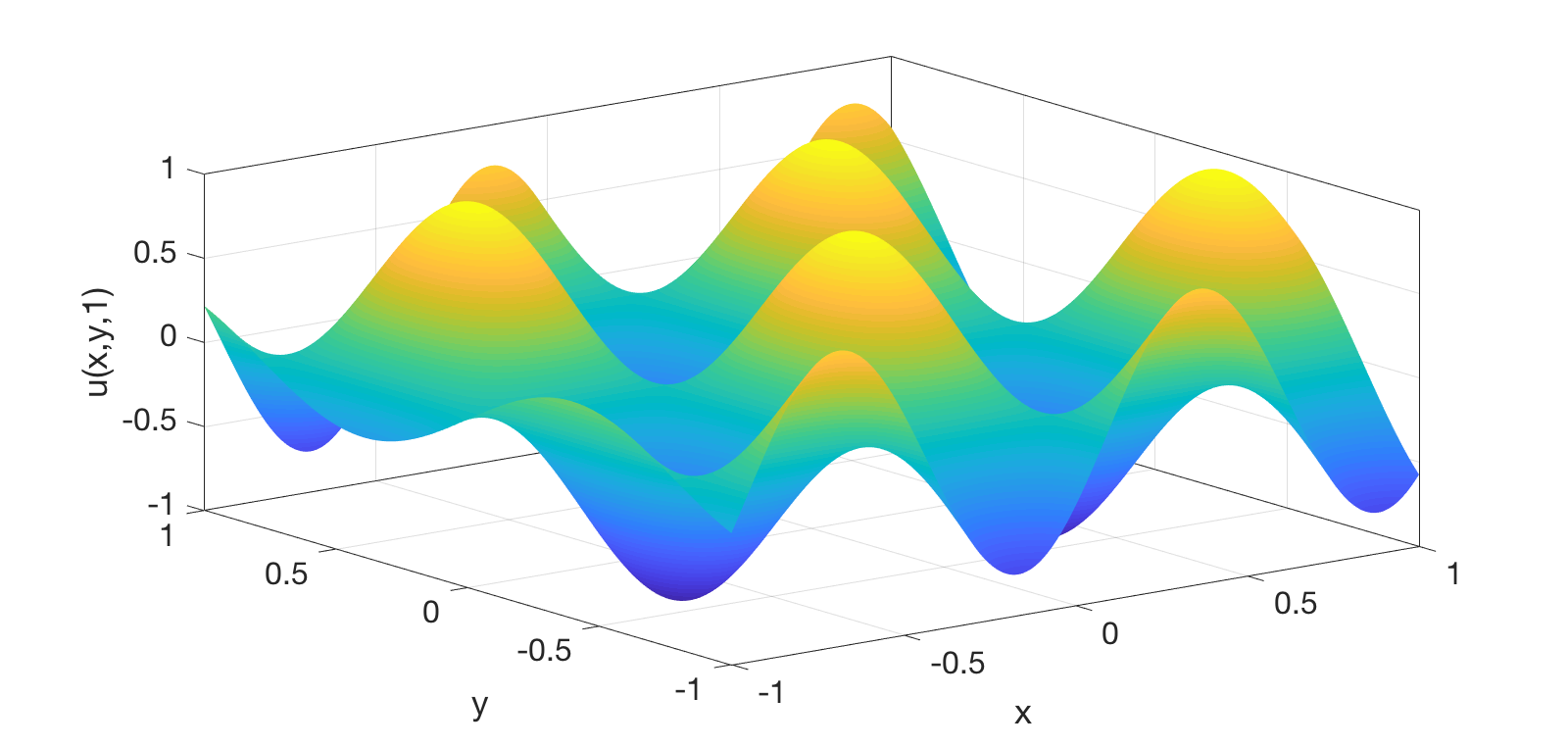
As an example, the following figures show the solution at time \(t=1\) and the convergence of the error for the manufactured wave problem with \(a(x,y) \equiv 1, \, \omega = 10, \, k_x = 6\), and \(k_y=4\).
|
|